Pygmt利用在线数据绘制地形图

                                                                                                   

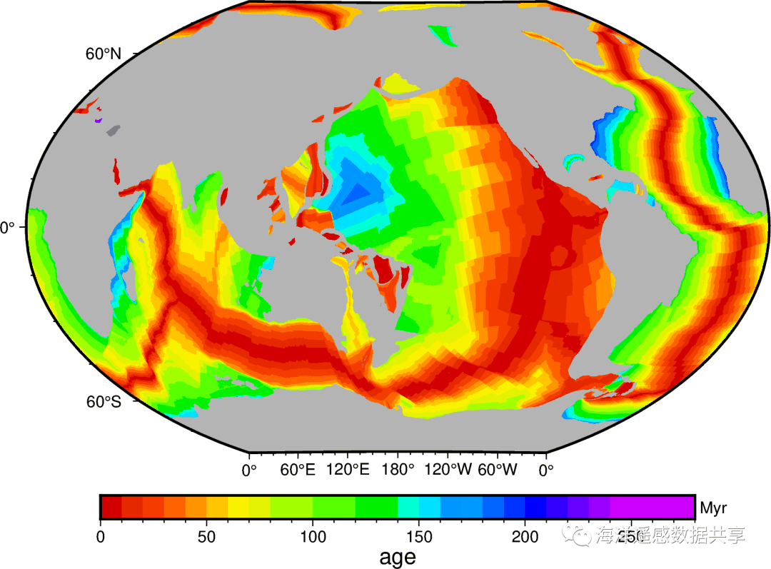
ＧＭＴ和Pygmt提供了一个远程数据功能，可以使用函数datasets远程下载多种在线数据，并进行处理和绘图。这里以pygmt为例绘制海底地壳年龄、陆地地形。

地壳数据[1]包含了不同的分辨率，对应不同文件大小，最粗为1d，全球数据仅125K，最大分辨率1m，全球数据188M。绘图

[C] 纯文本查看 复制代码

import pygmt
grid_globe = pygmt.datasets.load_earth_age(resolution='06m', region="-180/180/-90/90", registration=None)
fig = pygmt.Figure()
fig.grdimage(grid=grid_globe, projection="R15c", region="0/360/-89/89", frame=True,cmap="crustal_age.cpt")
fig.colorbar(frame=["af", "x+lage", "y+lMyr"],cmap="crustal_age.cpt")
fig.show()

$ V& z9 a& H& E) I
/ C8 T1 x2 K2 u* ^上面的调色板crustal_age可以在.gmt/cache/下找到，而远程数据也下载到了./gmt/server/下面。

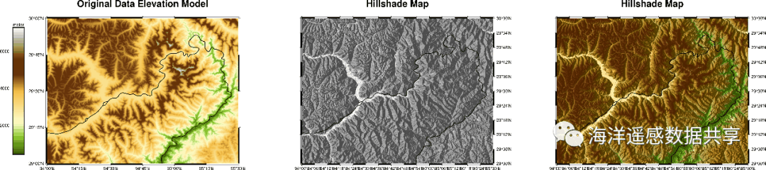
地形数据

地形数据[2]包含多种不同分辨率，对应不同的文件大小，最粗为1d，文件大小128k，最高分辨率为1s，文件大小达41G：

SRTM绘图

[C] 纯文本查看 复制代码

# 雅鲁藏布江大峡谷[/b]grid = pygmt.datasets.load_earth_relief(
    "03s",
    region=[94, 95.5, 29, 30],
    registration="gridline",
    use_srtm=True,
)

# calculate the reflection of a light source projecting from west to east
# (azimuth of 270 degrees) and at a latitude of 30 degrees from the horizon
dgrid = pygmt.grdgradient(grid=grid, radiance=[270, 30])

fig = pygmt.Figure()
fig.grdimage(grid=grid, projection="M15c", region=[94, 95.5, 29, 30], frame=['WSrt+t"Original Data Elevation Model"',"xa", "ya"],cmap="dem1")
fig.colorbar(position="JML+o1.8c/0c+w10c/0.9c",frame=["af", "y+lmeter"])
fig.coast(rivers="a/1p",borders="2/5,red")

# Shift plot origin of the second map by 12.5 cm in x direction
fig.shift_origin(xshift="20c")
pygmt.makecpt(cmap="gray", series=[-1.5, 0.3, 0.01])
fig.grdimage(
    grid=dgrid,
    projection="M15c",
    frame=['lSEt+t"Hillshade Map"', "xa0.1", "ya0.1"],
    cmap=True,
)
fig.coast(rivers="a/1p",borders="2/5,red")

# Shift plot origin of the second map by 12.5 cm in x direction
fig.shift_origin(xshift="20c")
fig.grdimage(
    grid=grid,
    shading=dgrid,
    projection="M15c",
    frame=['lSEt+t"Hillshade Map"', "xa0.1", "ya0.1"],
    cmap="dem1",
)
fig.coast(rivers="a/1p",borders="2/5,red")

fig.show(width="20c")
fig.savefig("srtm.png")

+ ?  Y7 l3 Y3 n3 K) O3 W" W

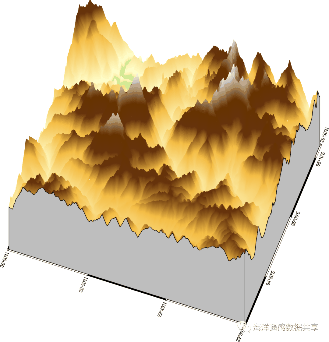
+ V& p! ?. K* h$ [2 f3 I3D地形图
7 i% |* _2 D$ ^

[C] 纯文本查看 复制代码

fig = pygmt.Figure()
fig.grdview(
    grid=grid,
    region=[94.7, 95.2, 29.5, 30],
    perspective=[250, 60],
    frame=["xa", "ya", "WSNE"],
    projection="M15c",
    zsize="15c",
    surftype="s",
    cmap="dem1",
    # Set the plane elevation to 1,000 meters and make the fill "gray"
    plane="000+ggray",
)

fig.show()

3 h  F& b# B) {5 K
# @5 n: [9 q9 L" {$ u% q" P, K% e

同样，我们还可以使用pygmt.grdview绘制三维地形图。下面是我曾经到过山脚下，但是在云中的南迦巴瓦峰。

4 c7 u5 U. i) ]/ V" w
$ s6 }2 C$ l9 \6 M! C
5 s( }5 o  h6 E# m8 z' I* l  C

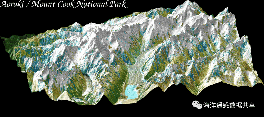
附：遥感影像和地形的结合

在github存在一个30Day*****的系列代码库，其中包含绘图领域的30DayMapChallenge2021，恰好已经使用GMT完成了这项工作，作者是Pygmt的核心开发者Weiji。

这里有两个遥感影像和地形结合的例子（17和18），可以作为很好的学习材料.

! ~9 [5 [4 ]9 [+ k+ ]

代码请前往：https://github.com/weiji14/30DayMapChallenge2021

References[1] 地壳数据: https://www.generic-mapping-tools.org/remote-datasets/earth-age.html
[2] 地形数据: https://www.generic-mapping-tools.org/remote-datasets/earth-relief.html

来源：海洋遥感数据共享
               
' Z6 g; x/ `$ j& p